Basic Ensemble Model in R
Overview
This project was designed to showcase the Ensemble Methodology for classification. Ensembles can provide better predictive capabilities than individual classification techniques; however, they come at the expense of increased processing power and time requirements. This is a proof of concept model that does not split the data into training and testing sets.
Library Necessary Packages
library(mlbench)        # Dataset

library(e1071)          # SVM, NB models
library(nnet)           # Neural Net model
library(rpart)          # RPart, LOOCV models
library(MASS)           # QDA model
library(klaR)           # RDA model
library(randomForest)   # Random Forest model
## randomForest 4.6-14
## Type rfNews() to see new features/changes/bug fixes.
library(caret) # Confusion Matrix
## Loading required package: lattice
## Loading required package: ggplot2
##
## Attaching package: 'ggplot2'
## The following object is masked from 'package:randomForest':
##
##     margin
library(ggplot2)        # Better Plots
library(rpart.plot)     # Better RPart Plots
library(wesanderson)    # Better Color Schemes
Load Data
This section imports the Breast Cancer dataset, omitting NA rows and removing the ID column, while keeping a copy of the IDs so they can be appended to the results table.
data(BreastCancer)
BreastCancer <- na.omit(BreastCancer)

BreastCancer.id <- BreastCancer[, 1]

BreastCancer <- BreastCancer[,-1]
Models
This section runs a variety of different classification models all which return a true or false classification.
Support Vector Machine Model
mysvm <- svm(Class ~ . , BreastCancer)
mysvm.pred <- predict(mysvm, BreastCancer)

length(mysvm.pred)
## [1] 683
length(BreastCancer$Class)
## [1] 683
table(mysvm.pred, BreastCancer$Class)
##
## mysvm.pred  benign malignant
##   benign       431         8
##   malignant     13       231
Naive Bayes Model
mynb <- NaiveBayes(Class ~ . , BreastCancer)
mynb.pred <- predict(mynb, BreastCancer)
table(mynb.pred$class, BreastCancer$Class)
##
##             benign malignant
##   benign       431         3
##   malignant     13       236
Neural Net Model
mynnet <- nnet(Class ~ . , BreastCancer, size = 1)
## # weights:  83
## initial  value 444.875707
## iter  10 value 70.908039
## iter  20 value 47.042231
## iter  30 value 38.495429
## iter  40 value 37.410696
## iter  50 value 33.178027
## iter  60 value 33.159982
## iter  70 value 32.581901
## iter  80 value 28.939637
## iter  90 value 28.933749
## iter 100 value 28.929784
## final  value 28.929784
## stopped after 100 iterations
mynnet.pred <- predict(mynnet, BreastCancer, type = "class")
table(mynnet.pred, BreastCancer$Class)
##
## mynnet.pred benign malignant
##   benign       441         2
##   malignant      3       237
Decision Tree Model
mytree <- rpart(Class ~ . , BreastCancer)
rpart.plot(mytree, box.palette = "GnRd")
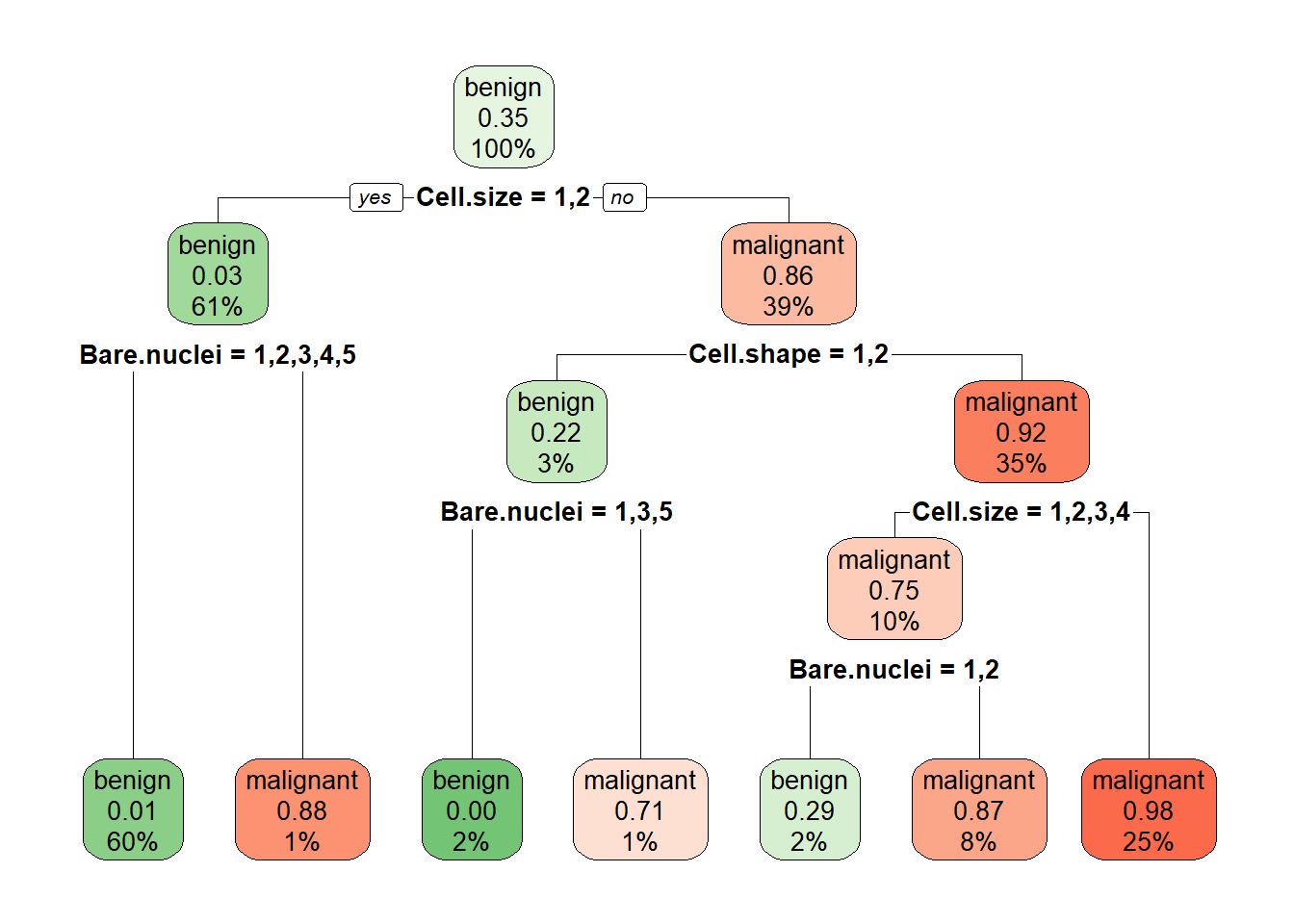
mytree.pred <- predict(mytree, BreastCancer, type = "class")
table(mytree.pred, BreastCancer$Class)
##
## mytree.pred benign malignant
##   benign       431         9
##   malignant     13       230
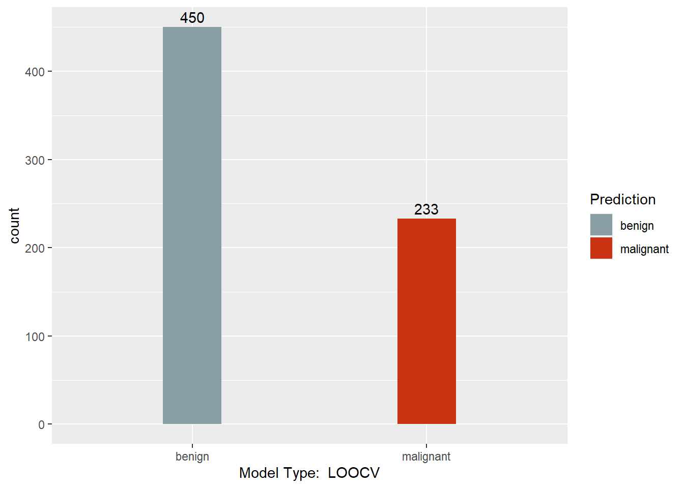
Leave-1-Out Cross Validation (LOOCV) Model
ans <- numeric(length(BreastCancer[, 1]))

for (i in 1:length(BreastCancer[, 1])) {
 myloocv <- rpart(Class ~ . , BreastCancer[-i, ])
 myloocv.pred <- predict(myloocv, BreastCancer[i, ], type = "class", se.fit = FALSE)
 ans[i] <- myloocv.pred
}

myloocv.pred <- factor(ans, labels = levels(BreastCancer$Class))
table(myloocv.pred, BreastCancer$Class)
##
## myloocv.pred benign malignant
##    benign       430        20
##    malignant     14       219
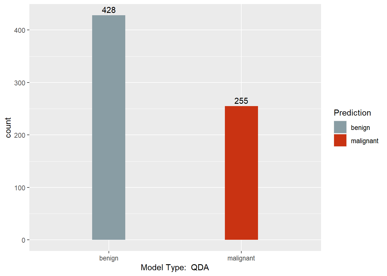
Quadratic Discriminant Analysis Model
BreastCancer.num <- BreastCancer

for(c in 1:ncol(BreastCancer.num)){
  BreastCancer.num[, c] <- cbind(as.numeric(BreastCancer.num[, c]))
}

myqda <- qda(Class ~ . , BreastCancer.num)
myqda.pred <- predict(myqda, BreastCancer.num)

table(myqda.pred$class, BreastCancer.num$Class)
##
##       1   2
##   1 422   6
##   2  22 233
Regularized Discriminant Analysis Model
myrda <- rda(Class ~ . , BreastCancer)
myrda.pred <- predict(myrda, BreastCancer)

table(myrda.pred$class, BreastCancer$Class)
##
##             benign malignant
##   benign       433         3
##   malignant     11       236
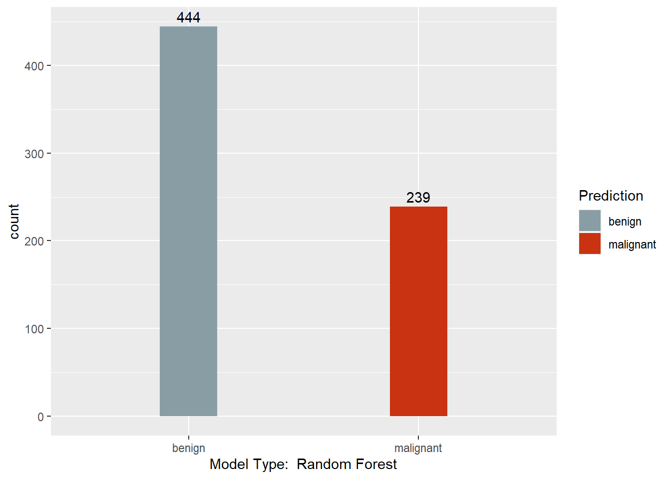
Random Forests Model
myrf <- randomForest(Class ~ . , BreastCancer)
myrf.pred <- predict(myrf, BreastCancer)
table(myrf.pred, BreastCancer$Class)
##
## myrf.pred   benign malignant
##   benign       444         0
##   malignant      0       239
Aggregate Predictions
This section combines predictions from all other sections into one dataframe. It then converts all columns to numeric to allow for a Majority Rule column to be created. This column calculates the average of each row’s values, then assigns a 1 or 2 based on whether the value is above or below 1.5. In the event of a tie (4 models with 1, 4 models with 2) the calculation takes the conservative approach of classifying as malignant.
Predictions.num <- data.frame(mysvm.pred, mynb.pred$class, as.factor(mynnet.pred), mytree.pred, myloocv.pred, myqda.pred$class, myrda.pred$class, myrf.pred)

for(c in 1:ncol(Predictions.num)){
  Predictions.num[, c] <- as.numeric(Predictions.num[, c])
}

denom <- ncol(Predictions.num)

Predictions.num$MajRule <- ifelse(rowSums(Predictions.num) / denom < 1.5, 1, 2)
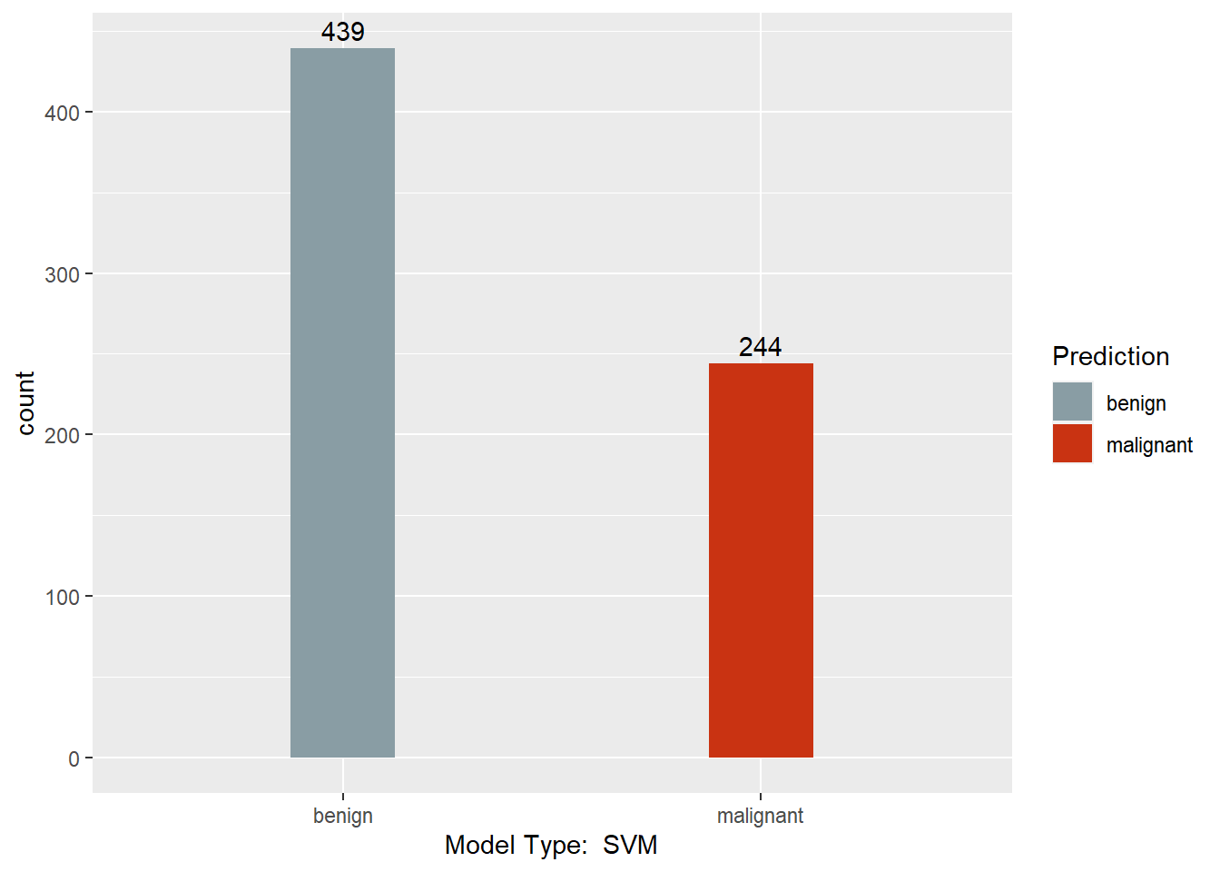
Output
This section converts the predictions back to factors, assigns names to each column of the Predictions dataframe, and creates a barchart with a count of each model’s predictions. Finally, a results dataframe is created that has the ID of the sample, and the majority prediction.
Predictions <- Predictions.num

prednames <- c("SVM", "Naive Bayes", "Neural Net", "Decision Tree", "LOOCV", "QDA", "RDA", "Random Forest", "Majority Vote")
type <- c("benign", "malignant")

for(c in 1:ncol(Predictions)){
  names(Predictions)[c] <- prednames[c]
  Predictions[, c] <- as.factor(Predictions[, c])
  levels(Predictions[, c]) <- type

  print(ggplot(data = Predictions,
               aes(x = Predictions[, c],
                   fill = Predictions[, c])) +
    geom_bar(width = 0.25) +
    scale_fill_manual(values = wes_palette(n = 3, name = "Royal1"), name = "Prediction") +
    xlab(paste("Model Type: ",
               prednames[c])) +
    geom_text(stat = 'count',
              aes(label = ..count..),
              vjust = -0.4,
              hjust = NA))
}


Results <- data.frame(BreastCancer.id, Predictions$`Majority Vote`)

confusionMatrix(Predictions$`Majority Vote`, BreastCancer$Class)
## Confusion Matrix and Statistics
##
##            Reference
## Prediction  benign malignant
##   benign       433         2
##   malignant     11       237
##
##                Accuracy : 0.981
##                  95% CI : (0.9677, 0.9898)
##     No Information Rate : 0.6501
##     P-Value [Acc > NIR] : <2e-16
##
##                   Kappa : 0.9585
##
##  Mcnemar's Test P-Value : 0.0265
##
##             Sensitivity : 0.9752
##             Specificity : 0.9916
##          Pos Pred Value : 0.9954
##          Neg Pred Value : 0.9556
##              Prevalence : 0.6501
##          Detection Rate : 0.6340
##    Detection Prevalence : 0.6369
##       Balanced Accuracy : 0.9834
##
##        'Positive' Class : benign
##
Lucas Forrest
CPA
My interests include data analytics, machine learning, and oddball computer projects.